TL;DR

I’ve been working on optimizing k-nearest neighbor (k-NN) search, and stumbled onto something interesting that I wanted to share.

The Problem

When you’re searching for the top-k most similar vectors in a large dataset, you end up performing a lot of distance calculations. In HNSW (Hierarchical Navigable Small World) graphs for example, you’re constantly comparing your query vector against candidate vectors to find the nearest neighbors.

Here’s the thing: once you’ve examined k candidates, you know the similarity threshold you need to beat. Any vector that can’t beat that threshold is useless to you. But traditionally, you only find out after you’ve performed the entire distance calculation.

For high-dimensional vectors (think 1536 or 2048 dimensions), that could be a lot of wasted computation.

Batched Early Abort

The optimization is conceptually simple: instead of computing the full distance in one shot, break it into batches of 16 dimensions at a time. After each batch, check if you can meet threshold. If you cannot possibly meet the threshold, bail out immediately.

// Pseudocode
// float distanceWithEarlyAbort(float* v1, float* v2, int dims, float threshold);
// Returns: partial distance (sum) if threshold exceeded, otherwise full distance
const int BATCH_SIZE = 16;
float sum = 0.0f;
for (int batch = 0; batch < dims; batch += BATCH_SIZE)
{
    sum += computeBatchDistance(v1, v2, batch, BATCH_SIZE);
    if (shouldAbort(sum, threshold))  // Comparison depends on metric (>, <, etc.)
    {
        return sum;  // Early abort - return partial distance
    }
}
return sum;  // Full distance computed

The key insight is that some distance calculations (L2 distance, LInf, DotProduct) are conducive to early aborts. So if part way through, you can determine that you cannot possibly meet the threshold, you can skip the rest.

Dynamic Threshold Updates

The other piece is keeping that threshold up to date. As the search progresses and you find better candidates, the threshold similarity changes. Push that updated threshold down to the distance calculation layer so it can abort even earlier.

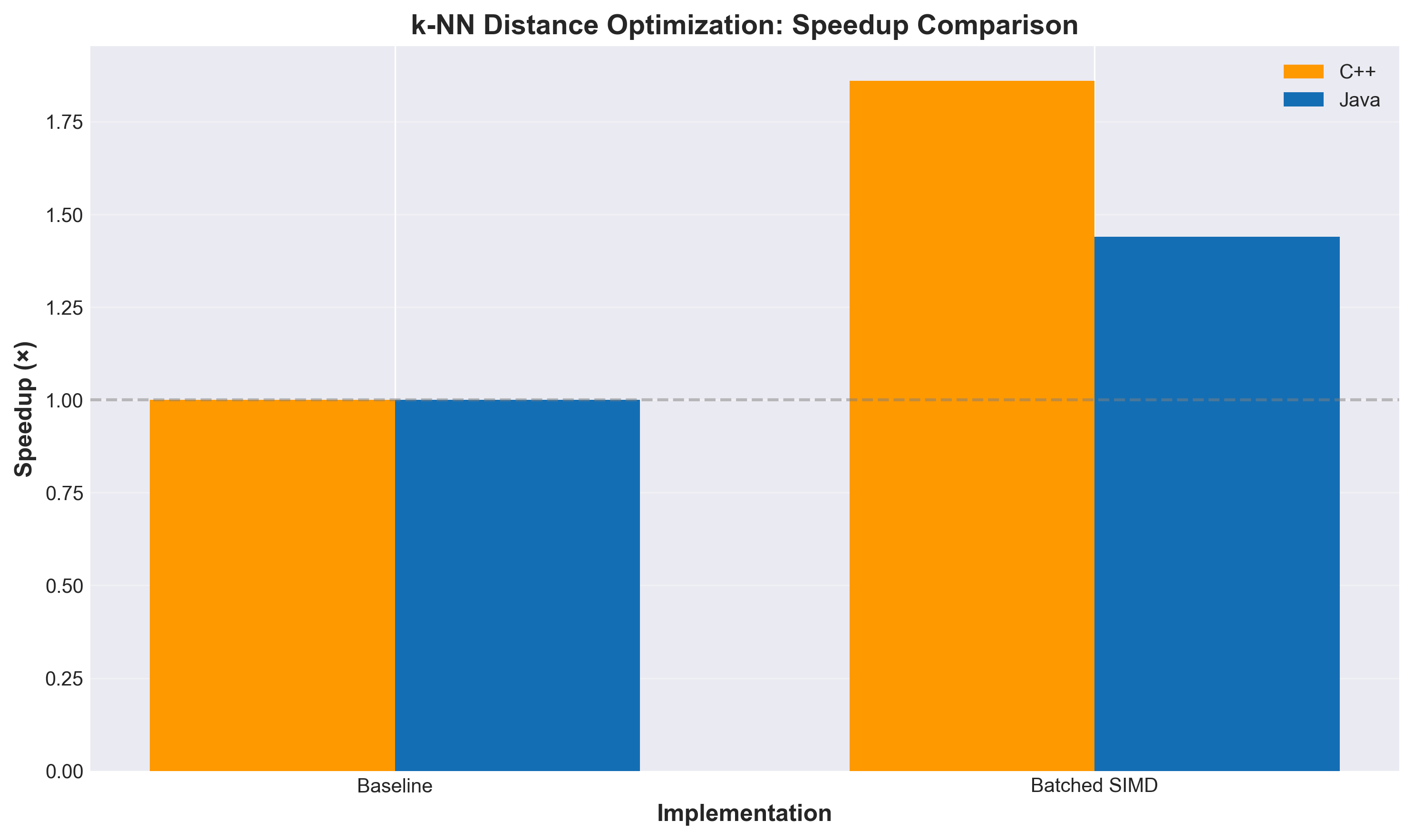
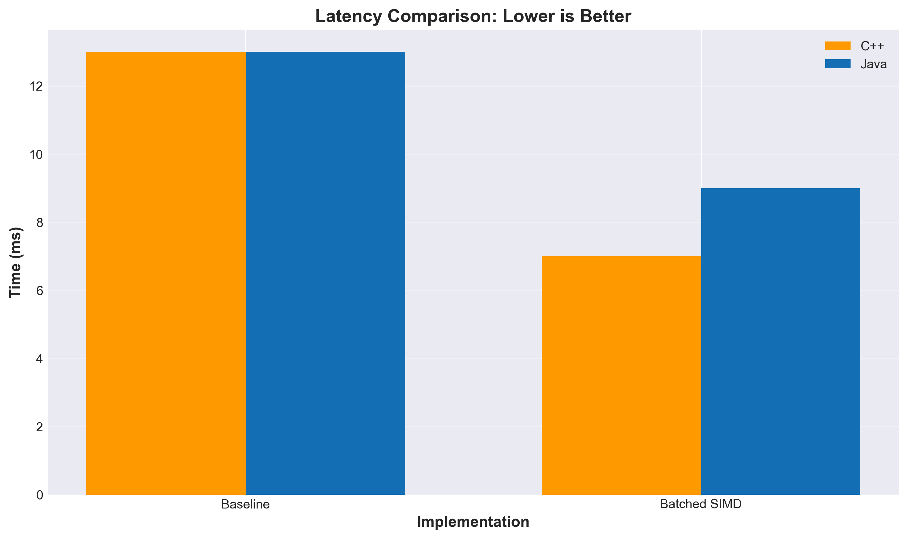
Results

Testing on 100K vectors with top-100 search:

The speedup gets better as dimensionality increases because there’s more opportunity to abort early. At 2048 dimensions, we’re seeing nearly 19× improvement.

Doing Less vs. Being Faster

There’s a fundamental distinction here that’s worth exploring: this optimization is about doing less work, not doing the same work faster.

When you optimize code with SIMD instructions, better algorithms, or compiler tricks, you’re making the CPU execute the same logical operations more efficiently. You’re still computing all 2048 dimensions—you’re just doing it faster with vector instructions that process multiple values per cycle.

Early abort is different. You’re literally skipping computation. If you abort after 512 dimensions because you can never meet the threshold, you never compute the remaining 1536 dimensions. The work simply doesn’t happen because it is an unnecessary waste.

The Unnecessary Work Problem: Computing Vector Modulus

Before we dive into the interaction with hardware, let’s talk about another form of unnecessary work that plagues vector search implementations: repeatedly computing vector norms.

Look at the cosine similarity formula:

cosine_similarity(x, y) = (x · y) / (||x|| * ||y||)

Where ||x|| is the L2 norm (modulus) of vector x: sqrt(sum(x_i^2)).

Now here’s the thing that drives me absolutely insane: most implementations compute these norms every single time they calculate cosine similarity. Every. Single. Time.

In NMSLIB’s cosine distance implementation, you’ll find code that computes sqrt(sum(x_i^2)) and sqrt(sum(y_i^2)) for every distance calculation. FAISS does the same thing in many of its distance functions—though to their credit, they provide normalize_L2() to pre-normalize vectors, effectively computing and storing the reciprocal of the norm by making ||x|| = 1.

But here’s what kills me: the norm of a vector doesn’t change. If you’re comparing a query vector against 100,000 database vectors, you’re computing the query vector’s norm 100,000 times. The exact same value. Over and over.

Why? Why are we doing this?

Some implementations have separate classes for normalized vs. non-normalized vectors, which is a step in the right direction. But even then, if your vectors aren’t normalized, you’re recomputing norms on every comparison.

Here’s what we should be doing:

1. Compute the norm once when you first encounter a vector
2. Pass it around as metadata alongside the vector
3. Store it on disk with the vector data
4. Never compute it again

Yes, this costs extra storage—4 whole bytes per vector for a float32 norm. For a million 1536-dimensional vectors, that’s 4MB of additional storage. The vectors themselves are 6GB. We’re talking about 0.07% storage overhead.

In exchange, you eliminate a square root and a number of multiply-add operations equal to the number of dimensions from every single distance calculation. For cosine similarity, you’re cutting the computational cost nearly in half.

And yet, implementation after implementation recomputes norms. It’s maddening.

If you’re building a vector search system and you are continually recomputing norms with your vectors, you’re leaving massive performance on the table. Precompute them. Store them. Pass them around. Treat them as first-class metadata.

This isn’t a clever optimization. This is basic algorithmic hygiene. We should have been doing this from day one. But, thank you, I’ll take credit for it. You heard it here first.

The Interaction with Hardware Acceleration

This gets interesting when you combine early abort with SIMD. Modern CPUs have vector units (AVX-512, ARM NEON, etc.) that can process multiple floating-point operations in parallel. Java’s Panama Vector API exposes this capability in a portable way.

Here’s what happens with pure SIMD optimization:

• Without SIMD: Process 2048 scalar operations sequentially
• With SIMD (AVX-512): Process 16 floats per instruction, so ~128 vector operations
• Speedup: ~8-10× (not quite 16× due to memory bandwidth, instruction overhead, etc.)

Now add early abort on top:

• With SIMD + early abort: Process batches of 16 dimensions, check threshold, potentially stop after 512 dimensions
  • Effective work: ~32 vector operations instead of 128
  • Combined speedup: ~19× (from doing less work AND doing it faster)

The key insight is that these optimizations multiply, not add. If SIMD gives you 8× and early abort lets you skip 75% of the work, you get 8 × 4 = 32× theoretical speedup (actual results vary due to overhead).

But there’s a cost to early abort: every threshold check introduces a branch, and branch misprediction has a real performance penalty. This is why batch size matters—checking after every 16 dimensions (the SIMD width) balances the benefit of aborting early against the cost of frequent branching. More on this in the branch prediction section below.

Language Runtime Considerations

The implementation language matters more than you might think.

C/C++: You have direct control over SIMD intrinsics and can hand-tune the early abort logic. The compiler won’t reorder your threshold checks or optimize them away. You get predictable performance, but you’re writing platform-specific code.

Java (with Panama Vector API): The JIT compiler is your friend and your enemy. It can optimize hot paths aggressively, but it might also decide to unroll loops in ways that interfere with early abort. The Vector API gives you portable SIMD, but the JIT needs time to warm up and optimize. In production, after JIT warmup, you get near-C++ performance. During startup or with cold code paths, not so much. If you are testing, make sure you warmup.

Python/NumPy: I haven’t looked closely at this but to the best of my understanding, you’re calling into native code (BLAS libraries) for the heavy lifting. Early abort is harder to implement because you lose control once you call into numpy.dot(). You’d need to implement the batched logic in Cython or call into a custom C extension. Whether there will be benefits or not, I’m not really sure.

Branch Prediction and the Cost of Checking

Every time you check if (sum > threshold), you’re introducing a branch. Modern CPUs are good at predicting branches, but they’re not perfect. If the branch is unpredictable (sometimes abort, sometimes continue), you pay a penalty for misprediction—the CPU has to flush its pipeline and restart.

This is why batch size matters. Check too frequently (every dimension), and branch misprediction overhead dominates. Check too infrequently (every 256 dimensions), and you miss opportunities to abort early. Batch size of 16 appears to be a sweet spot—maybe because it aligns with the SIMD width for AVX-512, and it checks often enough to abort early without excessive branching. Your mileage may vary; someone who knows more about CPU microarchitecture should probably opine on the optimal batch size.

Memory Bandwidth vs. Compute

High-dimensional vector operations are often memory-bound, not compute-bound. Loading 2048 floats from RAM takes time, even if the CPU can process them quickly. Early abort helps here too: if you abort after 512 dimensions, you’ve only loaded 2KB instead of 8KB. That’s less pressure on the memory subsystem, better cache utilization, and fewer cache misses.

On modern CPUs with large L3 caches, this matters less for single queries. But when you’re processing thousands of queries concurrently (typical in production), cache pressure is real. Reducing memory footprint per query means more queries fit in cache, which means better overall throughput.

The Threshold Update Dance

The dynamic threshold update adds another layer of complexity. As the search progresses and you find better candidates, you’re constantly updating the threshold. This means:

1. The threshold check becomes more aggressive over time (more likely to abort early)
2. Later distance calculations benefit more than earlier ones
3. The order in which you evaluate candidates matters

In HNSW graphs, you’re traversing the graph in a specific order based on the graph structure. The graph is designed to find good candidates quickly, which means the threshold tightens rapidly in the early stages of search. This is perfect for early abort—by the time you’re deep in the search, most candidates get rejected after just a few batches.

Why 19× and Not More?

You might wonder: if we’re skipping 75% of the work, why not 4× speedup? Why 19×?

The answer is that we’re not uniformly skipping 75% across all candidates. Some candidates are rejected immediately (after 16 dimensions), some after 512, some need the full 2048. The distribution depends on the data and the query.

The 19× speedup at 2048 dimensions suggests we’re aborting very early for most candidates. Back-of-the-envelope: if we’re computing an average of ~100-200 dimensions per candidate instead of 2048, that’s a 10-20× reduction in work. Add SIMD on top, and you get to 19×.

The other factor is overhead. There’s fixed cost per candidate: fetching the vector from memory, setting up the loop, checking the result. Early abort doesn’t eliminate that overhead, it just reduces the variable cost (the actual distance computation).

Implementation Notes

I implemented this in both NMSLIB and Apache Lucene. The NMSLIB implementation (PR #572) was done in C++ and served as the initial proof of concept. The Lucene implementation uses both scalar and SIMD (Panama Vector API) versions. The batched approach works with both, though SIMD gives you additional speedup on top of the early abort optimization.

The tricky part was integrating it cleanly into the existing HNSW search code without breaking backward compatibility. The solution uses a threshold-aware scoring interface that defaults to no-op for similarity functions that don’t support early abort.

Three commits:

1. Core batched distance functions with early abort
2. API integration with threshold-aware scoring
3. Dynamic threshold updates in the search loop

All tests passing. The code is available in my Lucene fork on the knn-opt branch.

A similar change for FAISS is currently in the works.

The Role of AI in This Work

This optimization didn’t spring fully formed from an AI prompt. It came from a lot of manual exploration, experimentation, and learning across multiple languages.

The Manual Discovery Phase

The initial idea came from reading the FAISS and NMSLIB codebases. I’m partial to C/C++, and these libraries have battle-tested implementations of vector search at scale. Studying how they handle distance calculations revealed opportunities for early termination that weren’t being fully exploited.

I started with NMSLIB, implementing the batched early abort in C++, then started playing with Faiss. Then I looked into Rust, then Java. What surprised me was how differently each language and runtime handled the same logical operations.

The scalar implementations performed wildly differently across languages. Java’s JIT compiler made optimization decisions that sometimes helped, sometimes hurt. Rust’s LLVM backend optimized aggressively but predictably. C++ gave me full control but required platform-specific tuning.

The runtime costs of instructions aren’t uniform. A branch misprediction costs more in one context than another. Memory access patterns matter differently depending on cache behavior. SIMD intrinsics have different latencies on different CPUs. Then there’s the complication of testing across hardware: a MacOS laptop with Apple Silicon, another with Intel, and production hardware that has Intel, AMD, and who knows what else. What works optimally on one platform might perform differently on another.

After much hand-tweaking and experimentation, I finally understood the core principles: batch size matters, threshold checking frequency is a tradeoff, and the interaction with SIMD is multiplicative. At that point, I could describe exactly what I needed to an AI assistant.

Enter Kiro

Once I had clarity on the requirements, I started iterating with Kiro. My experience is that initial exploration without AI tools, followed by AI-assisted implementation, is the most effective approach. This is my personal preference – I make no assertions that this is some kind of best practice. It works for me this way …

Correctness is critical. Optimization that produces wrong results is worse than no optimization. Kiro helped me write comprehensive tests—40 unit tests covering edge cases, boundary conditions, and correctness validation across different vector dimensions and similarity functions.

Kiro also reviewed my code and reasoned through the logic. I’d describe the invariants (“batched distance must equal full distance when threshold isn’t exceeded”), and Kiro would validate that the implementation maintained those invariants.

My code was messy. Multiple experiments, commented-out attempts, inconsistent naming, unused variables, debug print statements. The code in the final pull request was cleaned up using Kiro. I didn’t type it all that cleanly—I was focused on making it work correctly first.

Documentation and Communication

Several email correspondences, benchmark analysis, and this blog post were all produced with Kiro’s help. I had the data and the understanding, but translating that into clear communication takes time. Kiro accelerated that process significantly. I could, for example, describe a change in a prompt quite simply and Kiro would quickly perform the change – consistently.

I also use kiro-cli, the command-line interface for Kiro, which integrates directly into my terminal workflow. This blog post itself was cleaned up and polished using Kiro—the initial draft was much rougher, with inconsistent structure and (at times incomprehensible) explanations. Kiro helped simplify the language, tighten the prose and improve the flow.

The key insight: AI tools are force multipliers, not replacements. You need to understand the problem deeply first. Once you do, AI can help you implement faster, test more thoroughly, and communicate more clearly.

Other insight: I don’t like Kiro’s usage of the comma but I don’t want to have the Oxford Comma debate with Kiro – today.

Try It Yourself

I find these optimizations to be effective, but I’m no expert on CPU microarchitectures, the interplay between language compilers and JIT optimizers, memory subsystem behavior, or the countless other factors that impact real-world performance. I’d love your help validating this work and making it better for everyone.

The code is available in multiple places:

• NMSLIB: PR #572 (C++ implementation)
• Apache Lucene: My fork on the knn-opt branch (Java with SIMD)
• FAISS: Implementation in progress

If you’re working with vector search and high-dimensional data, please consider trying these changes. Test them on your workloads, your hardware, your data distributions. Tell me what works and what doesn’t.

A note for those maintaining forks of these libraries: if you don’t regularly pull upstream changes, you might miss optimizations like this. Consider reviewing these PRs and integrating them into your fork if they make sense for your use case.

This is an open call: help me validate that this works across different scenarios. Help identify edge cases I haven’t considered. Help optimize the batch size for different CPU architectures. Let’s make vector search faster for everyone.

Why This Matters

Vector search is everywhere now—semantic search, RAG systems, recommendation engines. These systems often run at massive scale, processing millions of queries. A 10-20× speedup translates directly to lower latency, higher throughput, and reduced infrastructure costs.

And let’s not forget the environmental impact. Less work means less heat, less power consumption, less cooling infrastructure. When you’re running vector search at scale—millions of queries across thousands of servers—a 10-20× reduction in computation translates to real energy savings. The ecological impact could be significant. Making our code more efficient isn’t just about performance and cost; it’s about sustainability.

There’s also the benefit on low powered devices (mobile, Raspberry Pi, …).